Dynamic Bayesian Predictive Stacking for Spatiotemporal Analysis

We provide a brief tutorial of the spFFBS package. Here we shows the implementation of the Dynamic Bayesian Predictive Stacking on synthetically generated data. For any further details please refer to (Presicce and Banerjee 2026). More examples, are available in documentation, and functions help.

Working packages

library(spFFBS)
library(spBPS)

Data generation

We generate data from the model detailed in Equation (1) (Presicce and Banerjee 2026), over a unit square.

# Dimensions
tmax <- 25
tnew <- 5
n    <- 150
q    <- 2
p    <- 2
u    <- 50

# Parameters
Sigma  <- matrix(c(1, -0.3, -0.3, 1), q, q)
phi <- 8
alfa <- 0.8
a <- ((1/alfa)-1)
V <- a*diag((n+u))

set.seed(1)
# Generate constant sinthetic data structure
coords <- matrix(runif((n+u) * 2), ncol = 2)
D <- spBPS:::arma_dist(coords)
K <- exp(-phi * D)
W <- rbind( cbind(diag(p), matrix(0, p, (n+u))), cbind(matrix(0, (n+u), p), K) )

# Prior information and initial state
m0     <- matrix(0, (n+u)+p, q)
C0 <- rbind( cbind(diag(0.005, p), matrix(0, p, (n+u))), cbind(matrix(0, (n+u), p), K) )
theta0 <- mniw::rMNorm(n = 1, Lambda = m0, SigmaR = C0, SigmaC = Sigma)

# Generate dynamic sinthetic data structure
G <- array(0, c((n+u)+p, (n+u)+p, tmax+tnew))
theta <- array(0, c((n+u)+p, q, tmax+tnew))
X <- array(0, c((n+u), p, tmax+tnew))
P <- array(0, c((n+u), (n+u)+p, tmax+tnew))
Y <- array(0, c((n+u), q, tmax+tnew))

set.seed(1)
for (t in 1:(tmax+tnew)) {
  if (t >= 2) {  
    
  G[,,t]     <- diag(p+n+u)
  theta[,,t] <- G[,,t] %*% theta[,,t-1] + mniw::rMNorm(n = 1, Lambda = m0, SigmaR = W, SigmaC = Sigma)
  X[,,t]     <- matrix(runif((n+u)*p), (n+u), p)
  P[,,t]     <- cbind(X[,,t], diag((n+u)))
  Y[,,t]     <- P[,,t] %*% theta[,,t] + mniw::rMNorm(n = 1, Lambda = matrix(0, (n+u), q), SigmaR = V, SigmaC = Sigma)
  } 
  else {
    
  G[,,t]     <- diag(p+n+u)
  theta[,,t] <- G[,,t] %*% theta0 + mniw::rMNorm(n = 1, Lambda = m0, SigmaR = W, SigmaC = Sigma)
  X[,,t]     <- matrix(runif((n+u)*p), (n+u), p)
  P[,,t]     <- cbind(X[,,t], diag((n+u)))
  Y[,,t]     <- P[,,t] %*% theta[,,t] + mniw::rMNorm(n = 1, Lambda = matrix(0, (n+u), q), SigmaR = V, SigmaC = Sigma)
  }
}

# Unobserved data
Yfuture <- Y[(1:n),,(tmax+1):(tmax+tnew)]
Ytilde <- Y[-(1:n),,]
thetatilde <- theta[-(1:(n+p)),,]
Xtilde <- X[-(1:n),,]
crdtilde <- coords[-(1:n),]
Dtilde   <- as.matrix(dist(crdtilde))
Ktilde   <- exp(-phi*Dtilde)

# Observed data
Y <- Y[(1:n),,1:tmax]
X <- X[(1:n),,]
P     <- P[(1:n),1:(n+p),]
G     <- G[1:(n+p), 1:(n+p),]
crd <- coords[1:n,]
D   <- as.matrix(dist(crd))
K   <- exp(-D)
W <- rbind( cbind(diag(p), matrix(0, p, n)), cbind(matrix(0, n, p), K) )
V <- a*diag((n))

Setting priors and hyperparameters

# Priors
m0     <- matrix(0, n+p, q)
C0 <- rbind( cbind(diag(0.005, p), matrix(0, p, n)), cbind(matrix(0, n, p), K) )
nu0 <- 3
Psi0 <- diag(q)
prior <- list("m" = m0, "C" = C0, "nu" = nu0, "Psi" = Psi0)

# hyperparameters values
alfa_seq <- c(0.7, 0.8, 0.9)
phi_seq <- c(6, 8, 9)
par_grid <- list(tau = alfa_seq, phi = phi_seq)

Dynamic BPS fit

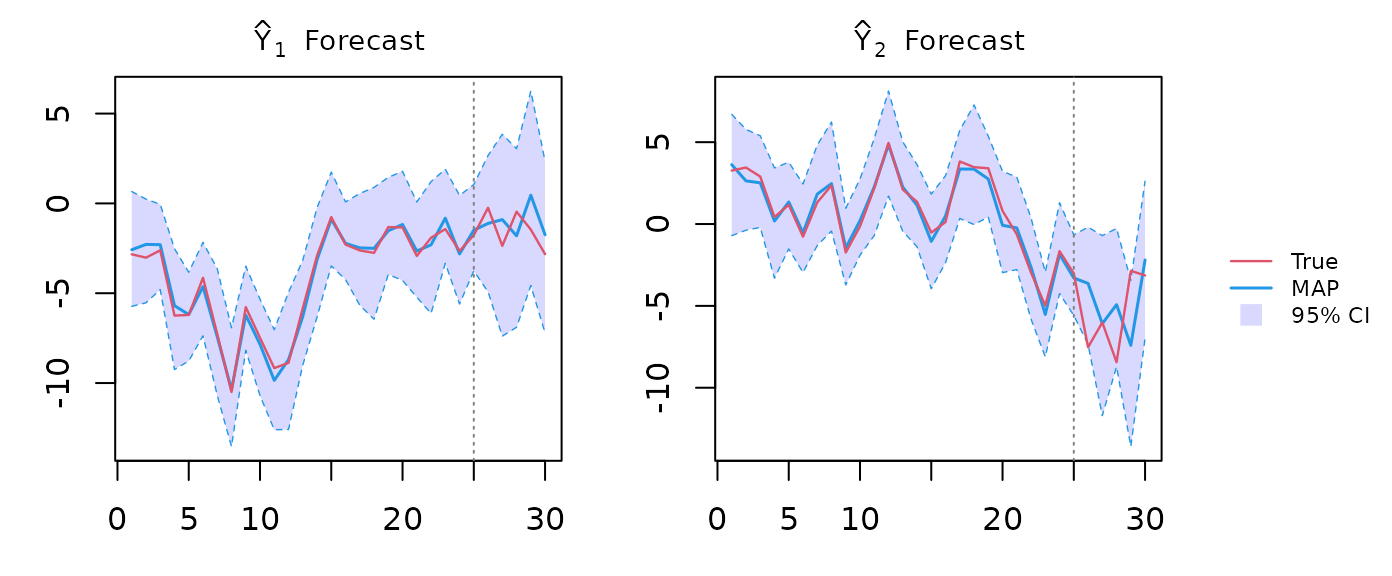
Posterior inference, forecast and spatial interpolation call (using 1 computing core):

out <- spFFBS::spFFBS(Y = Y, G = G, P = P, D = D,
                      grid = par_grid, 
                      prior = prior,
                      L = 200,
                      do_BS = T, 
                      do_forecast = T, 
                      tnew = tnew,
                      do_spatial = T,
                      spatial = list(crd = crd,
                                     crdtilde = crdtilde,
                                     Xtilde = Xtilde,
                                     t = tmax+tnew),
                      num_threads = 1)

Beta posterior inference

theta_post <- sapply(1:tmax, function(t){ out$BS[[t]] }, simplify = "array")
beta_post <- theta_post[1:p, 1:q,,]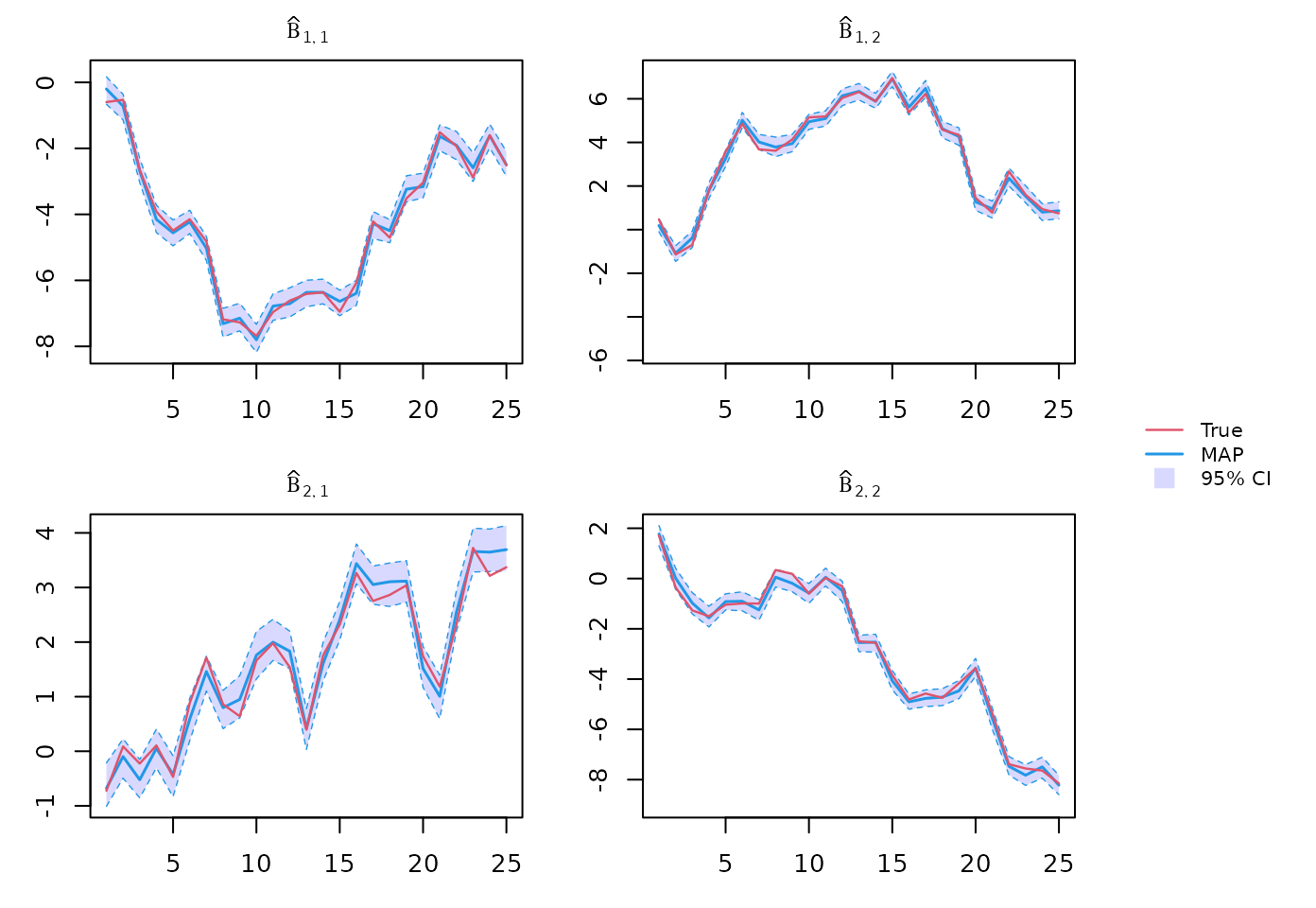

Sigma posterior inference

# Global weights
Wglobal <- out$Wglobal
J <- nrow(Wglobal)
L <- 200

# Posterior sampling
set.seed(1)
indL <- sample(1:J, L, Wglobal, rep = T)
Sigma_post <- sapply(1:L, function(l) {
  mniw::riwish(1, nu = out$FF[[tmax]]$filtered_results[[indL[l]]]$nu,
               Psi = out$FF[[tmax]]$filtered_results[[indL[l]]]$Psi) },
  simplify = "array")
Sigma_map <- apply(Sigma_post, c(1,2), median)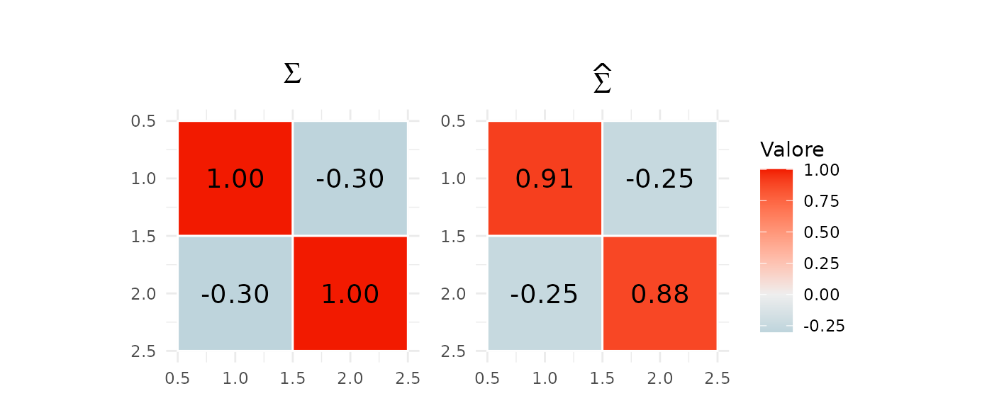

Multivariate outcome temporal forecasts

Y_forc <- out$forecast$Y_pred

Unobserved spacetime-points interpolation

Spatial interpolation for unobserved locations at future time points, here time point 30

Y_pred <- sapply(1:L, function(l){out$spatial[[1]][[l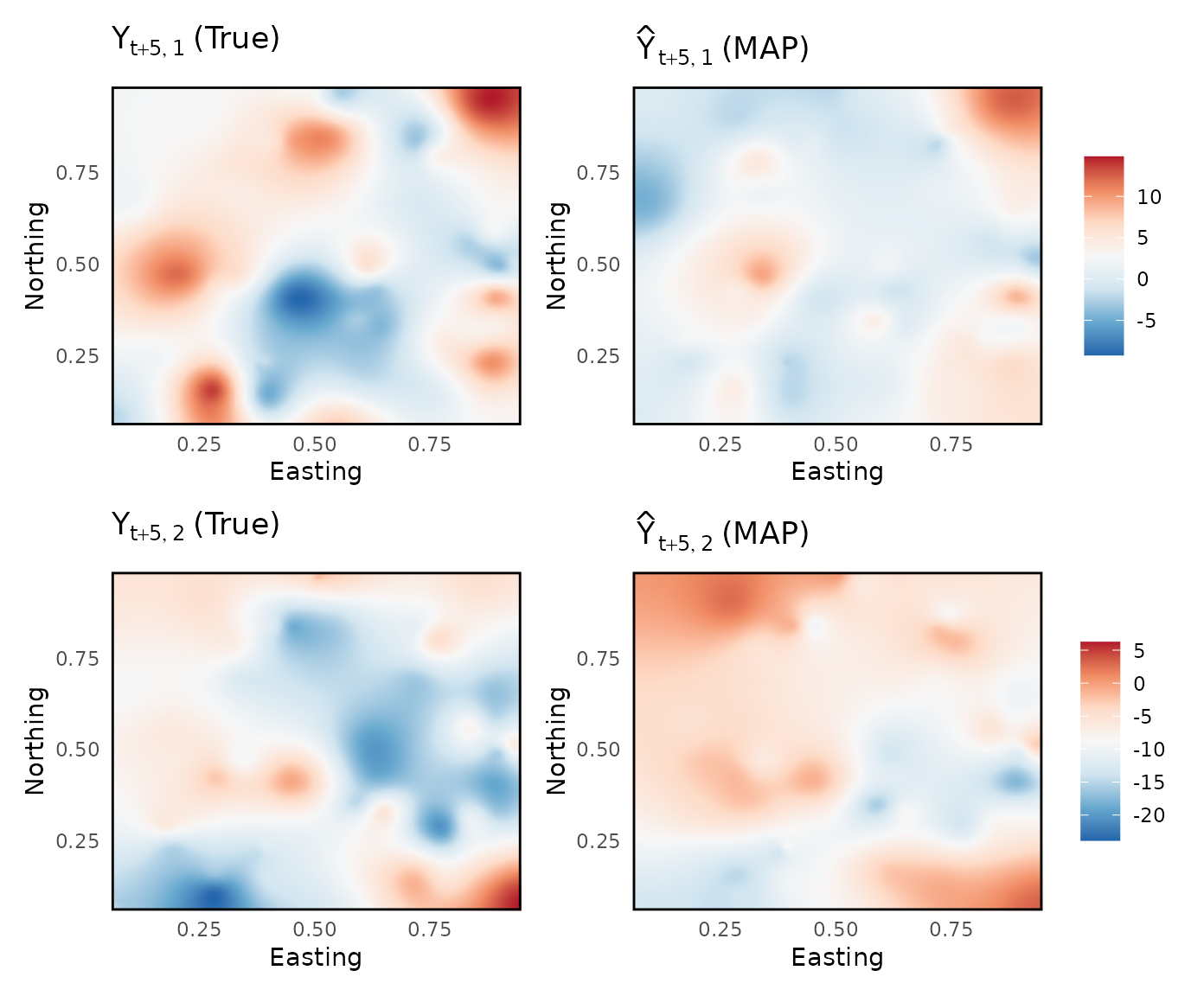]][1:u,]}, simplify = "array")

Presicce, Luca, and Sudipto Banerjee. 2026. “Adaptive Markovian Spatiotemporal Transfer Learning in Multivariate Bayesian Modeling.” arXiv Preprint, arXiv:2602.08544. https://doi.org/10.48550/arXiv.2602.08544.

Dynamic Bayesian Predictive Stacking for Spatiotemporal Analysis - Tutotial